The Classical Approach

Derivation of Parameters

Inverting the Mutual Induction Matrix

Representing Core and Winding Losses

Core Saturation

More on Air Core Reactance

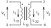
The theory of mutual coupling can be easily demonstrated using the coupling of two coils as an example.  This process can be extended to N mutually coupled windings as shown in References [1], [2] and [3]. For our purpose, consider the two mutually coupled windings as shown below:

Figure 6-1 - Two Mutually Coupled Windings

Where,

The voltage across the first winding is V1 and the voltage across the second winding is V2.  The following equation describes the voltage-current relationship for the two, coupled coils:

In order to solve for the winding currents, the inductance matrix needs to be inverted:

Where,

For 'tightly' coupled coils, wound on the same leg of a transformer core, the turns-ratio is defined as the ratio of the number of turns in the two coils. In an 'ideal' transformer, this is also the ratio of the primary and secondary voltages.  With voltages E1 and E2 on two sides of an ideal transformer, we have:

And

Making use of this turns-ratio 'a' Equation 6-1 may be rewritten as:

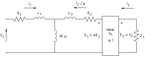
 Figure 6-2 - Equivalent Circuit of Two Mutually Coupled Windings

Where,

Now the inductance matrix parameters of Equation 6-1 can be determined from standard transformer tests, assuming sinusoidal currents. The self inductance of any winding 'x' is determined by applying a rated RMS voltage Vx to that winding and measuring the RMS current Ix flowing in the winding (with all other windings open-circuited). This is known as the open-circuit test and the current Ix is the magnetizing current. The self-inductance Lxx is given as:

Where,

Similarly, the mutual-inductance between any two coils 'x' and 'y' can be determined by energizing coil 'y' with all other coils open-circuited. The mutual inductance Lxy is then:

Transformer data is often not available in this format. Most often, an equivalent circuit, as shown in Figure 6-2, is assumed for the transformer and the parameters L1, L2 and aL12 are determined from open and short-circuit tests.

For example if we neglect the resistance in the winding, a short circuit on the secondary side (i.e. V2 = 0) causes a current to flow (assuming aL12 >> L2).  By measuring this current we may calculate the total leakage reactance L1 + L2. Similarly, with winding 2 open-circuited the current flowing is , from which we readily obtain a value for L1 + aL12.

Conducting a test with winding 2 energized and winding 1 open-circuited, . The nominal turns-ratio 'a' is also determined from the open circuit tests.

PSCAD computes the inductances based on the open-circuit magnetizing current, the leakage reactance and the rated winding voltages.

Derivation of Parameters

To demonstrate how the necessary parameters are derived for use by EMTDC, an example of a two winding, single-phase transformer is presented.  The data for the transformer is as shown in Table 6-1:

Table 6-1 - Transformer Data

If we ignore the resistances in Figure 6-1, we can obtain the (approximate) value for L1 + L2, from the short circuit test, as:

Where,

As no other information is available, we assume for the turns ratio 'a' the nominal ratio:

We also have for the primary and secondary base currents:

Thus, we see that by energizing the primary side with 100 kV, we obtain a magnetizing current:

But we also have the following expression from the equivalent circuit:

Where,

Therefore since,

Then,

By combining Equations 6-8 and 6-14 we obtain L1 = L2 =13.263 mH and from Equation 6-12 we obtain aL12 = 26.5119 H. The values for the parameters in Equation 6-1 are then obtained as:

Inverting the Mutual Induction Matrix

It was discussed previously that as the coefficient of coupling K approaches unity the elements of the inverse inductance matrix become large and approach infinity. This makes it impossible to derive the transformer currents in the form given by Equation 6-5.

An excessively small magnetising current also leads to such ill conditioning.  In such cases, it is often advisable to model the transformer with only leakage reactances and no magnetizing branch, as shown in Figure 6-3.  Such a transformer is referred to as 'ideal' in this document and also in PSCAD.

For an ideal transformer, the relationship between the derivatives of current (i.e. ) and the voltages can be directly expressed as in Equation 6-18; derived by considering the circuit equations for a short-circuit test conducted on one side, with a voltage source applied to the other (keep in mind that and either V1 or V2 is zero for a given test):

Where,

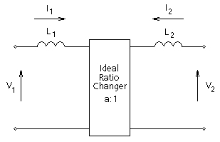
Figure 6-3 - 'Ideal' Transformer Equivalent Circuit

A similar analysis can be used to define the derivatives of the transformer currents in terms of its voltages for an 'ideal' transformer (i.e. zero magnetising current), when more than two windings are coupled on the same core.  

EXAMPLE 6-1

Consider a three winding, 40 MVA transformer with zero magnetising current.  The three-phase winding voltages are 230 kV, 66 kV and 13.8 kV.

An equivalent circuit diagram of the positive sequence leakage reactances is shown in Figure 6-4.  The inductances of the equivalent circuit are all based on the rated voltage of one winding, which for this example is winding 1 (the HV winding), rated at 132.79 kV ().  The LV winding rated voltage is 38.1 kV and the tertiary winding rated voltage is 13.8 kV.

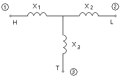
Figure 7-6 - Positive Sequence Leakage Reactance Equivalent Circuit

Where,

, ,  

and,

,  ,  

For a 60 hertz frequency rating, the inductance of leakage reactance X1 as shown above is found be the expression:

The leakage inductance values based on winding 1 voltage are therefore:

 ,   and  

As mentioned previously, the inverted inductance matrix of an 'ideal' three winding transformer is not as simple as that of an 'ideal' two winding transformer.  The inverted inductance matrix of an 'ideal' three winding transformer is given as follows:

Where,

Representing Core and Winding Losses

When an 'ideal' transformer is modeled, the magnetizing current is not represented and must be added separately.

Core losses are represented internally with an equivalent shunt resistance across each winding in the transformer.  These resistances will vary for each winding in order to maintain a uniform distribution across all windings. The value of this shunt resistance is based on the No Load Losses input parameter.

In most studies, core and winding losses can be neglected because of the little significance to results. Losses in the transmission system external to the transformer tend to dominate. Many transformer studies however, do require core saturation to be adequately modeled.  

Core Saturation

An exciting current is required for voltage transformation by a transformer. The excitation characteristic of a transformer is determined completely by the core design, and winding design affects the characteristic only in so far as it determines the flux density in the core. Transformers are constrained in their performance by the magnetic flux limitations of the core. Since ferromagnetic materials cannot support infinite magnetic flux densities and they tend to saturate at a certain level. The nonlinear flux-current characteristic of a transformer iron core is illustrated below.

Figure 6-5 - Flux-Current Characteristic of a Saturable Core Transformer

The transformer may experience saturation in any of the following situations:

• When a transformer's primary winding is overloaded from excessive applied voltage, the core flux may reach saturation levels during peak moments of the sinusoidal cycle. If this happens, the voltage induced in the secondary winding will no longer match the wave-shape as the voltage powering the primary coil. In other words, the overloaded transformer will distort the waveshape from primary to secondary windings, creating harmonics in the secondary winding's output.

• When a transformer is initially connected to an AC source, a transient current of up to 10 to 50 times larger than the rated transformer current can flow for several cycles. For large transformers, inrush current can last for several seconds. This happens because the transformer will always possess residual flux, and when the transformer is re-energized, the incoming flux will add to that already existing, which will cause the transformer to move into saturation. Then, only the resistance of the primary side windings and the power line itself limit the current.

Modeling Saturation Across a Specified Winding

In the classical transformer models, core saturation can be represented in one of two ways:  First, with a varying inductance across the winding wound closest to the core, or second, with a compensating current source across the winding wound closest to the core [2]. In EMTDC, the current source representation is used, since it does not involve change to (and inversion of) the subsystem matrix during saturation. For a two winding, single-phase transformer, saturation using a current source is shown below:

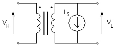
Figure 6-6 - Compensating Current Source for Core Saturation

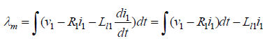
The current IS(t) is a function of winding voltage VL(t). First of all, winding flux lS(t) is defined by assuming that the current IS(t) in is the current in the equivalent non-linear saturating inductance LS(t) such that:

The non-linear nature of Equation 6-21 is displayed in Figure 6-6, where flux is plotted as a function of current.  The air core inductance LA is represented by the straight-line characteristic, which bisects the flux axis at lK. The actual saturation characteristic is represented by LM and is asymptotic to both the vertical flux axis and the air core inductance characteristic.  The sharpness of the knee point is defined by lM and IM, which can represent the peak magnetizing flux and current at rated volts. It is possible to define an asymptotic equation for current in the non-linear saturating inductance LS if LA, lK, lM, and IM are known.  Current IS can be defined as:

Where,

Figure 6-6 - Core Saturation Characteristic of the Classical Transformer

The flux lS(t) is determined as a function of the integral of the winding voltage VL(t) as follows:

This method is an approximate way to add saturation to mutually coupled windings.  More sophisticated saturation models are reported in literature, but suffer from the disadvantage that in most practical situations, the data is not available to make use of them - the saturation curve is rarely known much beyond the knee.  The core and winding dimensions, and other related details, cannot be easily found.

Studies in which the above simple model has been successfully used include:

• Energizing studies for a 1200 MVA, 500 kV, autotransformer for selecting closing resistors. Ranges of inrush current observed in the model compared favorably with the actual system tests.

• DC line AC converter bus fundamental frequency over-voltage studies.

• Core saturation instability where model results agreed closely to actual system responses [4].

In order to appreciate the saturation process described above, Figure 6-7 summarizes the use of Equations 6-22 and 6-23.

Figure 6-7 - Formulation of Saturation for a Mutually Coupled Winding (TSAT21)

Modeling Saturation Across the Magnetizing Inductance (Middle)

The approach of injecting the current source at the transformer terminal, as discussed above, usually provides acceptable simulation results for many large power system studies. However, the impact of voltage drops across the leakage impedance is significant during the saturation of transformer, since the magnetizing inductance will drop dramatically during the saturation. This phenomenon is not properly included in these models because the saturation current source location has been moved from its true location across the magnetizing impedance, to the new location across transformer terminal. To demonstrate the inaccurate results, two simulation cases that show the transformer inrush current in no load condition have been carried out. The transformer parameters are listed in Table 6-2.

Table 6-2 - Transformer Data

In the first simulation case the current source is placed at the primary winding terminal and in the second one it is at the secondary winding terminal. The simulation results of transformer magnetizing current and secondary voltage for both scenarios are shown in Figure 6-8a and 6-8b respectively.

Figure 6-8a - Primary and Secondary Voltages when the Saturation Current is Injected at the Primary Winding

Figure 6-8b - Primary and Secondary Voltages when the Saturation Current is Injected at the Secondary Winding

It can be observed above that when the saturation current is injected at the terminals where the source is connected, the secondary voltage waveform is not distorted since other elements modeling the transformer are linear. On the other hand, injecting the saturation current at the secondary winding increases the distortion in its voltage waveform. This phenomena is also true for three and four winding transformer models.

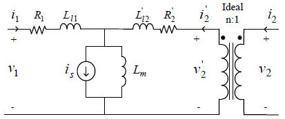
Figure 6-9 - Transformer T-Model Including Saturation Current at the Middle

Figure 6-9 shows the true location of magnetizing branch in the transformer T model. The magnetizing current can be divided into two components; the linear component which is represented as a linear inductance defined as:

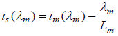
where λM and IM are the peak magnetizing flux and current at rated voltage as shown in Figure 6-6, and the nonlinear component that is the difference between the total magnetizing current and the linear current as illustrated in Figure 6-10. The nonlinear component or saturation current can be calculated as follows:

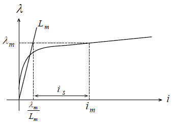
Figure 6-10 - Magnetizing Current Consists of Linear Current and Saturation Current

In Equation 6-25, im is the total magnetizing current and lm is the magnetizing flux calculated by:

In this method of saturation modeling, the location of the saturation branch should be maintained at the terminals of the transformer in order to retain the computational efficiency. Therefore the true saturation current is partitioned between the terminal current sources by appropriate ratios as shown in Figure 6-11. To do so, the injected currents at both terminals should be accurately computed to be mathematically equivalent to injection at the magnetizing branch so that the new model behaves exactly the same as the transformer T model.

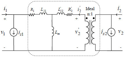
Figure 6-11 - Mathematically Equivalent Model of Transformer Electric Circuit

The simulation results of the secondary voltage of the same case mentioned above in Figure 6-8, using the new model, along with the previous simulations for the placement of the saturation at either ends is presented in Figure 6-12.

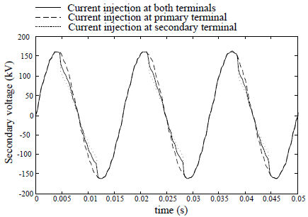
Figure 6-12 - Mathematically Equivalent Model of Transformer Electric Circuit

For more details on this saturation method, please see transformer reference [12].

More on Air Core Reactance

The air core reactance LA in Figure 6-6 may not be known for a transformer under study. One rule of thumb is that air core reactance is approximately twice the leakage reactance.

For example, if the saturation is applied to the tertiary winding of the three winding transformer, a reasonable value to select for air core reactance would be XHT, which is 24%.  Thus, as seen from the tertiary, the air core reactance would be 24%; as seen from the low voltage winding is would be 38%, and as seen from the high voltage winding it would be 48% or twice the leakage reactance XHT.

The knee point of the saturation curve is sometimes available and is usually expressed in percent or per-unit of the operating point, defined by rated voltage.  Typical ranges in per-unit are 1.15 to 1.25.  Referring to Figure 6-6, this would be:

Where,

1.15 < K < 1.25

If the RMS rated voltage of the winding, across which saturation is applied, is VM, then lM is:

Where,

Equations 6-21 to 6-25 are an approximate means of defining transformer saturation and form the basis upon which the EMTDC subroutine TSAT21 is constructed.