Development of the PSCAD Line Constants Program (or LCP) is based on the work of a variety of scientists and engineers in the field of transmission systems over the past few decades, and contains some of the most relevant modeling techniques in the industry today (see References [18], [23] for example). The primary purpose of the LCP is to calculate all frequency domain parameters (or constants) required, so that distributed transmission systems can be convolved into two-port, time domain representations and interfaced with the EMTDC network. Whether modeling the system at a single frequency or performing a full frequency-dependent representation, the LCP will execute the necessary steps to arrive at the required constants.
The present form of the LCP (originally released with PSCAD V3) is actually an amalgamation of two programs that existed in PSCAD V2: T-LINE and CABLE. It now exists as a separate executable file placed along with the PSCAD executable in the installation directory, and is called by PSCAD whenever a transmission system is encountered. Although the two T-LINE and CABLE programs are now merged together, the LCP still requires that aerial and underground systems not be combined. That is, underground cables and overhead transmission lines must be designed and solved separately. This is mainly due to the fact that the calculation of ground return impedance in both systems is fundamentally different, and there is presently no means by which to efficiently represent the mutual effects between the two system types.
All input data is read by the LCP from either a transmission line or cable input file (*.tli or *.cli). The input file is generated automatically by PSCAD when a project is compiled, based on the system cross-section in the Transmission Segment Definition Editor (see the next section called Data Input). The LCP output constants are written to either a transmission line or cable output file (*.tlo or *.clo), which is then read in by EMTDC before the simulation begins. The output file contains pre-formatted data to help EMTDC construct a two-port network equivalent for the system. A log file (*.log) and a user output file (*.out) are also generated by the LCP.
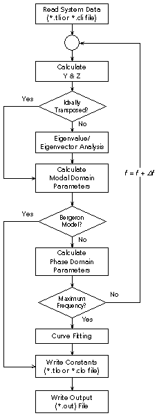
The LCP is structured as illustrated in Figure 9-2. All events outlined in this diagram are described in detail later in this chapter.
Figure 8-2: Basic PSCAD Line Constants Program Structure
The Line Constants Program is controlled through the use of a graphical user interface tool in PSCAD called the Transmission Segment Definition Editor. Within this tool, the user may define the transmission system by constructing a cross-section of the right-of-way, complete with conductor/cable positions, etc. This information is compiled by PSCAD when the constants are solved for that line, and written to a transmission line or cable input file (*.tli or *.cli) as mentioned previously.
The following list is a summary of the input parameters required by the LCP, some are referred to during discussions later in this chapter:
General:
|
Symbol |
Description |
|
|
Line length [km] |
|
|
Steady-state frequency [Hz] |
|
|
Number of conductors |
|
|
Ground resistivity [Wm] |
|
|
Ground relative permeability |
Aerial Lines:
|
Symbol |
Description |
|
|
Number of circuits |
|
|
Number of bundles/phases per circuit |
|
|
Number of sub-conductors per bundle |
|
|
Bundled conductor spacing (symmetrical only) [m] |
|
|
Horizontal position of tower in right-of-way [m] |
|
|
Sub-conductor horizontal position relative to [m] |
|
|
Sub-conductor height above the ground plane [m] |
|
|
Conductor/bundle horizontal position relative to xt [m] |
|
|
Conductor/bundle height above the ground plane [m] |
|
|
Conductor radius (sub-conductor radius if bundled) [m] |
|
|
Conductor DC resistance [W/km] |
|
|
Conductor sag at midpoint between tower spans [m] |
|
|
Conductor shunt conductance [S/m] |
|
|
Ground wire horizontal position relative to xt [m] |
|
|
Ground wire height above the ground plane [m] |
|
|
Ground wire radius [m] |
|
|
Ground wire DC resistance [W/km] |
|
|
Ground wire sag at midpoint between tower spans [m] |
Underground Cables:
|
Symbol |
Description |
|
|
Number of cables |
|
|
Number of conducting layers per cable |
|
|
Conductor inner radius [m] |
|
|
Conductor outer radius [m] |
|
|
Conductor resistivity [Wm] |
|
|
Conductor relative permeability |
|
|
Insulator relative permittivity |
|
|
Insulator relative permeability |
|
|
Horizontal position of cable in right-of-way [m] |
|
|
Cable depth below surface of ground plane [m] |
The geometric position of overhead conductors or cable centres in a transmission system cross-section, are ultimately input to the LCP in terms of Cartesian coordinates (i.e. linear x and y dimensions). These coordinates are relative to a reference point in both the x and y direction. The ground plane is considered the reference level (y = 0.0) in the y direction, and the x reference is an arbitrary point that is defined through data entry in the tower or cable cross-section components (xt in Figure 8-3).
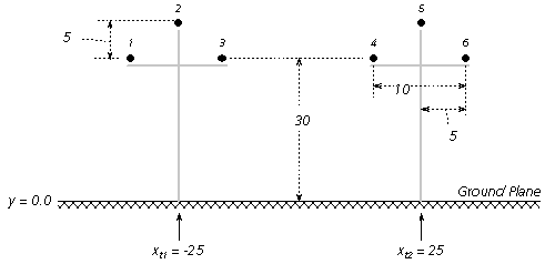
Figure 8-3: x and y References in a Typical Overhead Line Cross-Section
NOTE: Although underground y-coordinates for cables are below the y = 0.0 plane, they are still entered as positive values.
The LCP allows conductor xy position data to be entered either directly, or in a relative manner through tower dimensions, such as horizontal and vertical distances between conductors and relative x position of the tower. The latter option is provided as transmission line tower data is often given in this format. If the user desires to enter the coordinates directly, then the Universal Tower component is provided in the PSCAD Master Library.
For example, the system in Figure 8-3 consists of two towers and six conductors. A set of xy coordinates for each conductor is derived given the tower input data so that (assuming both towers are structurally identical):
|
|
|
|
|
|
|
|
|
|
|
|
|
|
|
|
|
|
NOTE: Conductor positions must be considered carefully when entering the data, otherwise erroneous results will be given. The LCP contains some sanity checks to ensure that conductors or cables do not overlap; however there is no way to check for incorrect conductor position!
Sag is a phenomena associated with suspended conductors, which tend to droop under their own weight when strung between tower stands. The amount of sag present is dependent not only on conductor weight, but also on tower span length, conductor properties and ambient temperature. Temperatures can vary considerably, depending on environmental conditions and power demand.
The Line Constants Program approximates the affects of conductor sag by simply decreasing the effective conductor height above ground by a factor of 2/3 of the total sag.
|
|
(8-1) |
The approximation eliminates sag by assuming a conductor of uniform height y’. This effectively makes the calculation of constants, for a particular right of way, independent of tower span.
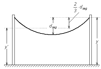
Figure 8-4: Setting Conductor Effective Height Given Sag